Published in the blogpost track of the ELLIS Workshop on Geometry-grounded Representation Learning and Generative Modeling at ICML 2024. Written by Patrick Feeney and Michael C. Hughes.
Contrastive learning encompasses a variety of methods that learn a constrained embedding space to solve a task. The embedding space is constrained such that a chosen metric, a function that measures the distance between two embeddings, satisfies some desired property, usually that small distances imply a shared class. Contrastive learning underlies many self-supervised methods, such as MoCo (He et al., 2020), (Chen et al., 2021), SimCLR (Chen et al., 2020), (Chen et al., 2020), and BYOL (Grill et al., 2020), as well as supervised methods such as SupCon (Khosla et al., 2020) and SINCERE (Feeney and Hughes, 2024).
In contrastive learning, there are two components that determine the constraints on the learned embedding space: the similarity function and the contrastive loss. The similarity function takes a pair of embedding vectors and quantifies how similar they are as a scalar. The contrastive loss determines which pairs of embeddings have similarity evaluated and how the resulting set of similarity values are used to measure error with respect to a task, such as classification. Backpropagating to minimize this error causes a model to learn embeddings that best satisfy the constraints induced by the similarity function and contrastive loss.
This blog post examines how similarity functions and contrastive losses affect the learned embedding spaces. We first examine the different choices for similarity functions and contrastive losses. Then we conclude with a brief case study investigating the effects of different similarity functions on supervised contrastive learning.
Similarity Functions
A similarity function \(s(z_1, z_2): \mathbb{R}^d \times \mathbb{R}^d \rightarrow \mathbb{R}\) maps a pair of \(d\)-dimensional embedding vectors \(z_1\) and \(z_2\) to a real similarity value, with greater values indicating greater similarity. A temperature hyperparameter \(0 < \tau \leq 1\) is often included, via \(\frac{s(z_1, z_2)}{\tau}\), to scale a similarity function. If the similarity function has a range that is a subset of \(\mathbb{R}\), then \(\tau\) can increase that range. \(\tau\) is omitted for simplicity here.
Cosine Similarity
A common similarity function is cosine similarity
This function measures the cosine of the angle between \(z_1\) and \(z_2\) as a scalar in \([-1, 1]\). Cosine similarity violates the triangle inequality, making it the only similarity function discussed here that is not derived from a distance metric.
Negative Arc Length
The recently proposed negative arc length similarity function (Koishekenov et al., 2023) provides an analogue for cosine similarity that is a distance metric
This function assumes that \(||z_1|| = ||z_2|| = 1\) which is a common normalization (Le-Khac et al., 2020) that restricts the embeddings to a hypersphere. The arc length \(\text{arccos}(z_1 \cdot z_2)\) is a natural choice for comparing such vectors as it is the geodesic distance, or the length of the shortest path between \(z_1\) and \(z_2\) on the hypersphere. Subtracting the arc length converts the distance metric into a similarity function with range \([0, 1]\).
Negative Euclidean Distance
The negative Euclidean distance similarity function is simply
Euclidean distance measures the shortest path in Euclidean space, making it the geodesic distance when \(z_1\) and \(z_2\) can take any value in \(\mathbb{R}^d\). In this case the similarity function has range \([-\infty, 0]\).
The negative Euclidean distance can also be used with embeddings restricted to a hypersphere, resulting in range \([-2, 0]\). However, this is not the geodesic distance for the hypersphere as the path being measured is inside the sphere. The Euclidean distance will be less than the arc length unless \(z_1 = z_2\), in which case they both equal 0.
Contrastive Losses
A contrastive loss function maps a set of embeddings and a similarity function to a scalar value. Losses are written such that derivatives for backpropagation are taken with respect to the embedding \(z\).
Margin Losses
The original contrastive loss (Chopra et al., 2005) maximizes similarity for examples \(z^+\) and minimizes similarity for examples \(z^-\), until the similarity is below margin hyperparameter \(m\), via
The structure of this loss implies that \(z_1\) and \(z_2\) share a class if \(s(z_1, z_2) < m\) and otherwise they do not share a class. This margin hyperparameter can be challenging to tune for efficiency throughout the training process because it needs to be satisfiable but also provide \(z^-\) samples within the margin in order to backpropagate the error.
The triplet loss (Schroff et al., 2015) avoids this by using a margin between similarity values
The triplet loss only updates a network when its loss is positive, so finding triplets satisfying that condition are important for learning efficiency.
Lifted Structured Loss (OhSong et al., 2016) handles this by precomputing similarities for all pairs in a batch then selecting the \(z^-\) with maximal similarity
The Batch Hard loss (Hermans et al., 2017) takes this even further by selecting \(z^+\) with minimal similarity
The decision to compute the loss based on comparisons between \(z\), a single \(z^+\), and a single \(z^-\) comes with advantages and disadvantages. These methods can be easier to adapt for learning with varying levels of supervision because complete knowledge of whether similarity should be maximized or minimized for each pair in the dataset is not required. However, these methods also make training efficiently difficult and provide relatively loose constraints on the embedding space.
Cross Entropy Losses
A common contrastive loss is the Information Noise Contrastive Estimation (InfoNCE) (Oord et al., 2019) loss
InfoNCE is a cross entropy loss whose logits are similarities for \(z\). \(z^+\) is a single embedding whose similarity with \(z\) should be maximized while \(z^-_1, z^-_2, \ldots, z^-_n\) are a set of \(n\) embeddings whose similarity with \(z\) should be minimized. The structure of this loss implies that \(z_1\) shares a class with \(z_2\) if no other embedding has greater similarity with \(z_1\).
The choice of \(z^+\) and \(z^-\) sets varies across methods. The self-supervised InfoNCE loss chooses \(z^+\) to be an embedding of an augmentation of the input that produced \(z\) and \(z^-\) to be the other inputs and augmentations in the batch. This is called instance discrimination because only augmentations of the same input instance have their similarity maximized.
Supervised methods expand the definition of \(z^+\) to also include embeddings which share a class with \(z\). The expectation of InfoNCE loss over choices of \(z^+\) is used to jointly maximize their similarity to \(z\). The Supervised Contrastive (SupCon) loss (Khosla et al., 2020) uses all embeddings not currently set as \(z\) or \(z^+\) as \(z^-\), including embeddings that share a class with \(z\) and therefore will also be used as \(z^+\). This creates loss terms that would minimize similarity between embeddings that share a class. Supervised Information Noise-Contrastive Estimation REvisited (SINCERE) loss (Feeney and Hughes, 2024) removes embeddings that share a class with \(z\) from \(z^-\), leaving only embeddings with different classes. An additional margin hyperparameter can also be added to these losses (Barbano et al., 2022), which allows for interpolation between the original losses and losses with the \(e^{s(z, z^+)}\) term removed from the denominator.
Considering a set of similarities during loss calculation allows the loss to implicitly perform hard negative mining (Khosla et al., 2020), avoiding the challenge of selecting triplets required by a margin loss. The lack of a margin places strict constraints on the embedding space, as similarities are always being pushed towards the maximum or minimum. This enables analysis of embedding spaces that minimize the loss. For example, InfoNCE and SINCERE losses with cosine similarity are minimized by embedding spaces with clusters of inputs mapped to single points (maximizing similarity) that are uniformly distributed on the unit sphere (minimizing similarity) (Wang and Isola, 2020).
Case Study: Contrastive Learning on a Hypersphere
Many modern contrastive learning techniques build off of the combination of cosine similarity and cross entropy losses. However, few papers have explored changing similarity functions and losses outside of the context of a more complex model.
Koishekenov et al. (2023) recently reported improved downstream performance by replacing cosine similarity with negative arc length for two self-supervised cross entropy losses. This change is motivated by the desire to use the geodesic distance on the embedding space, which in this case is a unit hypersphere. We investigate whether replacing cosine similarity with negative arc length similarity can improve performance with the SINCERE loss, which is supervised, and how each similarity affects the learned embedding space.
Supervised Learning Accuracy
We utilize the methodology of Feeney and Hughes (2024) to evaluate if the results of Koishekenov et al. (2023) generalize to supervised cross entropy losses. Specifically, we train models with SINCERE loss and each similarity function then evaluate the models with nearest neighbor classifiers on the test set.
| CIFAR-10 | CIFAR-100 | |||
| Similarity | 1NN | 5NN | 1NN | 5NN |
| Cosine | 95.88 | 95.91 | 76.23 | 76.13 |
| Negative Arc Length | 95.66 | 95.65 | 75.81 | 76.41 |
We find no statistically significant difference based on the 95% confidence interval of the accuracy difference (Foody, 2009) from 1,000 iterations of test set bootstrapping. This aligns with the results in Feeney and Hughes (2024), which found a similar lack of statistically significant results across choices of supervised contrastive cross entropy losses. This suggests that supervised learning accuracy is similar across choices of reasonable similarity functions and contrastive losses.
Supervised Learning Embedding Space
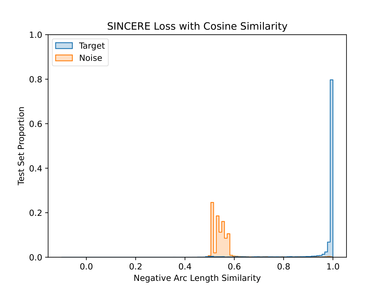
We also visualize the learned embedding space for each CIFAR-10 model. For each test set image, the similarity value is plotted for the closest training set image that shares a class (“Target”) and that does not share a class (“Noise”). This visualizes the 1-nearest neighbor decision process. Both similarity functions are plotted for each model, with the title denoting the similarity function used during training.
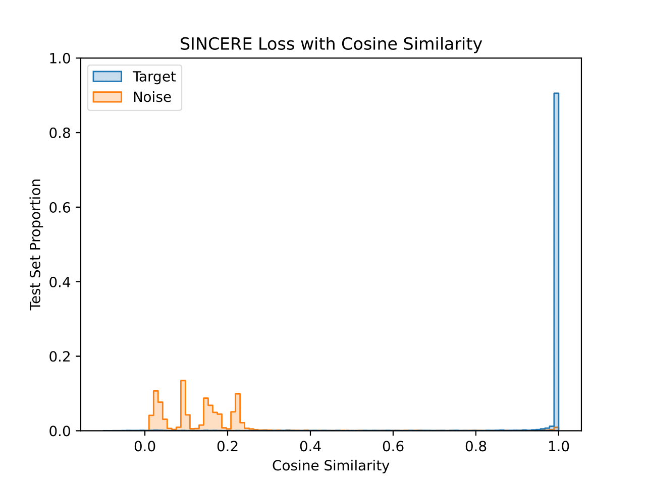
The model trained with cosine similarity maximizes the similarity to target images well. There are a small number of noise images with near maximal similarity, but the majority are below 0.3 cosine similarity. Interestingly, the peaks seen in the noise similarity reflects the fact that individual classes will have different modes of their noise histograms.
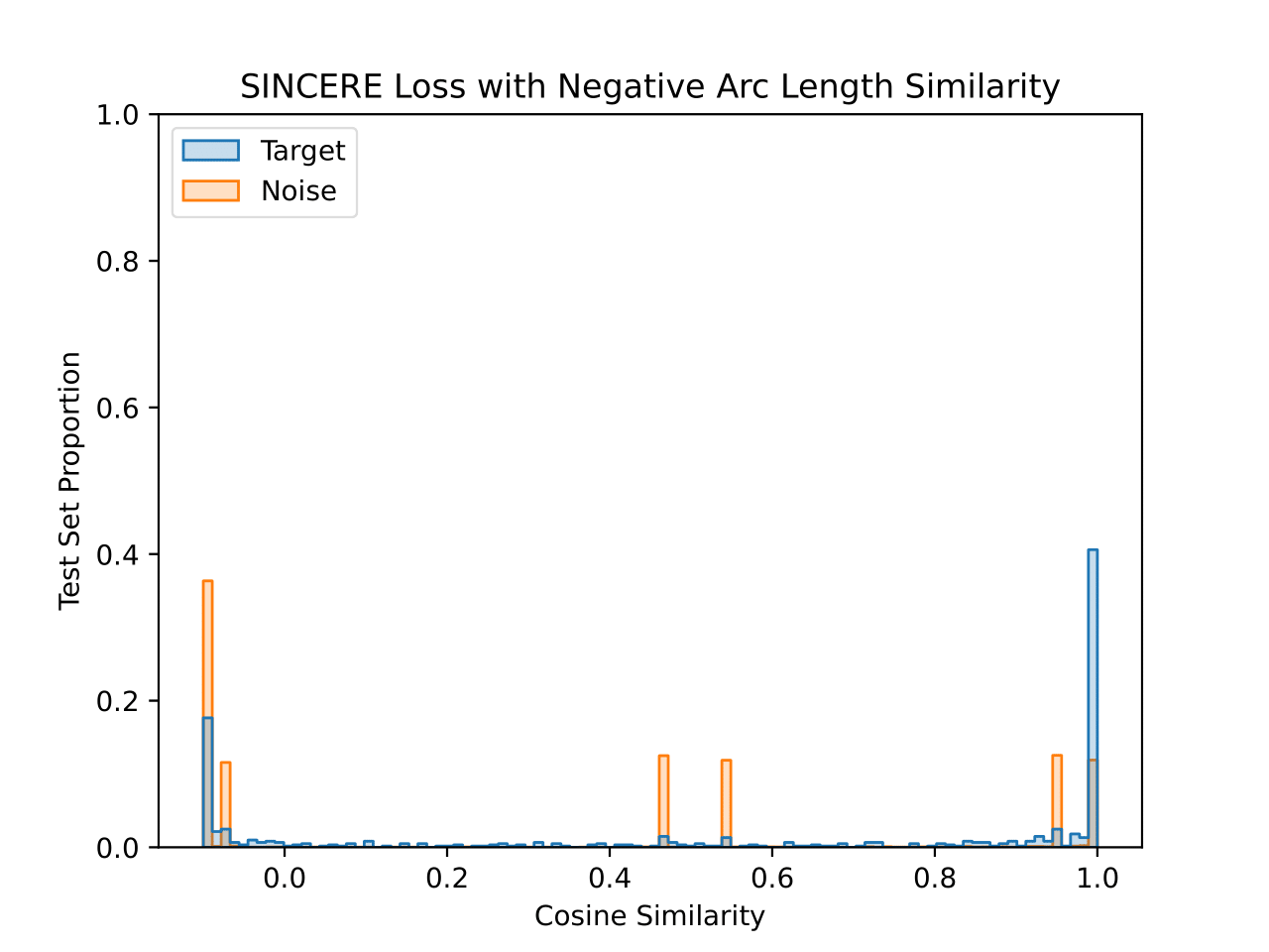
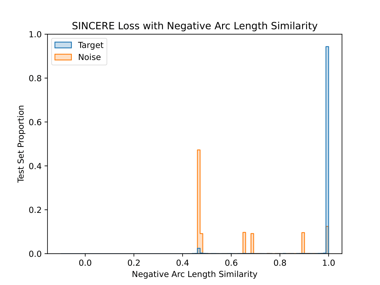
The model trained with negative arc length similarity does a better job of forcing target similarity values very close to 1 negative arc length similarity, but also has a notable number of target similarities near 0.5 negative arc length similarity. The noise distribution also reflects the fact that individual classes have different modes for their noise histograms, but in this case the modes are spread across more similarity values. Notably the peak for the horse class is very close to the max similarity due to a high similarity to the dog class, although they are still separated enough from the target similarities to not have an impact on accuracy.
Discussion
The choice of similarity function clearly has an effect on the learned embedding space despite a lack of statistically significant changes in accuracy. The cosine similarity histogram most cleanly aligns with the intuition that contrastive losses should be maximizing and minimizing similarities. In contrast, the negative arc length similarity histogram suggests similarity minimization is sacrificed for very consistent maximization. These differences in the learned embedding spaces could affect performance on downstream tasks such as transfer learning.
Bibliography
Carlo Alberto Barbano, Benoit Dufumier, Enzo Tartaglione, Marco Grangetto, and Pietro Gori. Unbiased supervised contrastive learning. In The Eleventh International Conference on Learning Representations. September 2022. URL: https://openreview.net/forum?id=Ph5cJSfD2XN (visited on 2024-05-28). ↩
Ting Chen, Simon Kornblith, Mohammad Norouzi, and Geoffrey Hinton. A simple framework for contrastive learning of visual representations. In Proceedings of the 37th International Conference on Machine Learning, 1597–1607. PMLR, November 2020. ISSN: 2640-3498. URL: https://proceedings.mlr.press/v119/chen20j.html (visited on 2023-02-07). ↩
Ting Chen, Simon Kornblith, Kevin Swersky, Mohammad Norouzi, and Geoffrey E Hinton. Big self-supervised models are strong semi-supervised learners. In Advances in Neural Information Processing Systems, volume 33, 22243–22255. Curran Associates, Inc., 2020. URL: https://proceedings.neurips.cc/paper/2020/hash/fcbc95ccdd551da181207c0c1400c655-Abstract.html (visited on 2023-07-28). ↩
Xinlei Chen, Saining Xie, and Kaiming He. An empirical study of training self-supervised vision transformers. In Proceedings of the IEEE/CVF International Conference on Computer Vision, 9640–9649. 2021. URL: https://openaccess.thecvf.com/content/ICCV2021/html/Chen_An_Empirical_Study_of_Training_Self-Supervised_Vision_Transformers_ICCV_2021_paper.html (visited on 2023-02-09). ↩
S. Chopra, R. Hadsell, and Y. LeCun. Learning a similarity metric discriminatively, with application to face verification. In 2005 IEEE Computer Society Conference on Computer Vision and Pattern Recognition (CVPR'05), volume 1, 539–546 vol. 1. June 2005. ISSN: 1063-6919. URL: https://ieeexplore.ieee.org/abstract/document/1467314?casa_token=fbldvqZUi0gAAAAA:sIzRPsJfUiIGmux-j7j6aoov1PNxo944AwjVUdSzTh47MueCdAM3fLFyFf20oLu2lr33z_ph (visited on 2024-05-28), doi:10.1109/CVPR.2005.202. ↩
Patrick Feeney and Michael C. Hughes. Sincere: supervised information noise-contrastive estimation revisited. February 2024. arXiv:2309.14277 [cs]. URL: http://arxiv.org/abs/2309.14277 (visited on 2024-03-20), doi:10.48550/arXiv.2309.14277. ↩ 1 2 3 4
Giles M. Foody. Classification accuracy comparison: hypothesis tests and the use of confidence intervals in evaluations of difference, equivalence and non-inferiority. Remote Sensing of Environment, 113(8):1658–1663, August 2009. URL: https://www.sciencedirect.com/science/article/pii/S0034425709000923 (visited on 2024-05-28), doi:10.1016/j.rse.2009.03.014. ↩
Jean-Bastien Grill, Florian Strub, Florent Altché, Corentin Tallec, Pierre Richemond, Elena Buchatskaya, Carl Doersch, Bernardo Avila Pires, Zhaohan Guo, Mohammad Gheshlaghi Azar, Bilal Piot, koray kavukcuoglu, Remi Munos, and Michal Valko. Bootstrap your own latent - a new approach to self-supervised learning. In Advances in Neural Information Processing Systems, volume 33, 21271–21284. Curran Associates, Inc., 2020. URL: https://proceedings.neurips.cc/paper/2020/hash/f3ada80d5c4ee70142b17b8192b2958e-Abstract.html (visited on 2023-03-08). ↩
Kaiming He, Haoqi Fan, Yuxin Wu, Saining Xie, and Ross Girshick. Momentum contrast for unsupervised visual representation learning. In Proceedings of the IEEE/CVF Conference on Computer Vision and Pattern Recognition, 9729–9738. 2020. URL: https://openaccess.thecvf.com/content_CVPR_2020/html/He_Momentum_Contrast_for_Unsupervised_Visual_Representation_Learning_CVPR_2020_paper.html (visited on 2023-02-07). ↩
Alexander Hermans, Lucas Beyer, and Bastian Leibe. In defense of the triplet loss for person re-identification. November 2017. arXiv:1703.07737 [cs]. URL: http://arxiv.org/abs/1703.07737 (visited on 2024-05-28), doi:10.48550/arXiv.1703.07737. ↩
Prannay Khosla, Piotr Teterwak, Chen Wang, Aaron Sarna, Yonglong Tian, Phillip Isola, Aaron Maschinot, Ce Liu, and Dilip Krishnan. Supervised contrastive learning. In Advances in Neural Information Processing Systems, volume 33, 18661–18673. Curran Associates, Inc., 2020. URL: https://proceedings.neurips.cc/paper_files/paper/2020/hash/d89a66c7c80a29b1bdbab0f2a1a94af8-Abstract.html (visited on 2024-03-20). ↩ 1 2 3
Yeskendir Koishekenov, Sharvaree Vadgama, Riccardo Valperga, and Erik J. Bekkers. Geometric contrastive learning. In 2023 IEEE/CVF International Conference on Computer Vision Workshops (ICCVW), 206–215. Paris, France, October 2023. IEEE. URL: https://ieeexplore.ieee.org/document/10350974/ (visited on 2024-04-26), doi:10.1109/ICCVW60793.2023.00028. ↩ 1 2 3
Phuc H. Le-Khac, Graham Healy, and Alan F. Smeaton. Contrastive representation learning: a framework and review. IEEE Access, 8:193907–193934, 2020. URL: https://ieeexplore.ieee.org/document/9226466/ (visited on 2023-11-09), doi:10.1109/ACCESS.2020.3031549. ↩
Hyun Oh Song, Yu Xiang, Stefanie Jegelka, and Silvio Savarese. Deep metric learning via lifted structured feature embedding. In Proceedings of the IEEE Conference on Computer Vision and Pattern Recognition, 4004–4012. 2016. URL: https://www.cv-foundation.org/openaccess/content_cvpr_2016/html/Song_Deep_Metric_Learning_CVPR_2016_paper.html (visited on 2024-05-28). ↩
Aaron van den Oord, Yazhe Li, and Oriol Vinyals. Representation learning with contrastive predictive coding. January 2019. arXiv:1807.03748 [cs, stat]. URL: http://arxiv.org/abs/1807.03748 (visited on 2024-05-28), doi:10.48550/arXiv.1807.03748. ↩
Florian Schroff, Dmitry Kalenichenko, and James Philbin. Facenet: a unified embedding for face recognition and clustering. In Proceedings of the IEEE Conference on Computer Vision and Pattern Recognition, 815–823. 2015. URL: https://www.cv-foundation.org/openaccess/content_cvpr_2015/html/Schroff_FaceNet_A_Unified_2015_CVPR_paper.html (visited on 2024-05-28). ↩
Tongzhou Wang and Phillip Isola. Understanding contrastive representation learning through alignment and uniformity on the hypersphere. 2020. ↩